After benchmarking your application and concluding that the performance is insufficient, the next step is profiling. Profiling measures where execution time is spent so that we can focus our optimization effort on parts of the code where it will have the most impact. This scientific approach is typically much more effective than guessing.

Sampling vs tracing

This article will discuss sampling (statistical) profiling. The program is stopped repeatedly to record the callstack. If this is done enough times then we get an idea of where the CPU spends its time. This method is different to tracing, where an entry is recorded every time an event occurs, such as on entry to or return from a function. Typically sampling profiling has lower overhead and is more useful for analyzing throughput or bandwidth, whereas tracing is more useful for analyzing latency or IO problems.

Recording a profile

We can record a profile with:

probe-rs profile --duration 200 <executing-elf-file> callstack --cores 0 --rate 1 naive-dwarf

Replace <executing-elf-file> with a path to the ELF file executing on the device. This will sample core 0 at 1Hz for 200 seconds using DWARF debug information to unwind callstacks. The output will be written to probe-rs-profile.json.gz, visualizing this is discussed in a later section.

Overhead and number of samples

We halt the CPU to collect each sample, this means that high sampling rates can cause a lot of overhead, as the CPU spends a large fraction of time halted. This overhead can particularly be a problem for programs that interact with the outside world¹. This overhead likely varies with the speed of your microcontroller and debug probe. It can be useful to benchmark your application while profiling in order to check that the overhead is not too high.

The standard error on our measurements is the square root of the count for each measurement. If we measure 5 samples in a function then our expected error is roughly 45%. If we measure 100 samples in a function our expected error is 10%.

We should adjust the duration and rate to ensure that we get reasonable statistics and low overhead.

Callstack method

As of writing two methods are available to recover the callstacks for recording:

• naive-dwarf
• naive-frame-pointer

Details on both methods can be found in this blog post.

Both methods require enabling debug information, for example by modifying the release profile in Cargo.toml:

[profile.release]
debug = 2

naive-frame-pointer additionally requires frame pointers to be enabled when compiling the target binary. This can be done by setting RUSTFLAGS:

RUSTFLAGS="-C force-frame-pointers=yes" cargo build --release

or by adding lines under the [build] or [target.'xyz'] section of the .cargo/config.toml:

rustflags = [
  # enable frame pointers for profiling
  "-C", "force-frame-pointers=yes",
]

Displaying a profile

We use samply to display the generated profile. It can be installed with:

cargo install --locked samply

Then to display our generated profile:

samply load probe-rs-profile.json.gz

This will open the profile in firefox profiler in your browser. samply will continue running to convert program addresses to function names and display code listings when queried. Switching to the “Flame Graph” tab, double clicking a bar and clicking the “asm” button yields a view like the following:

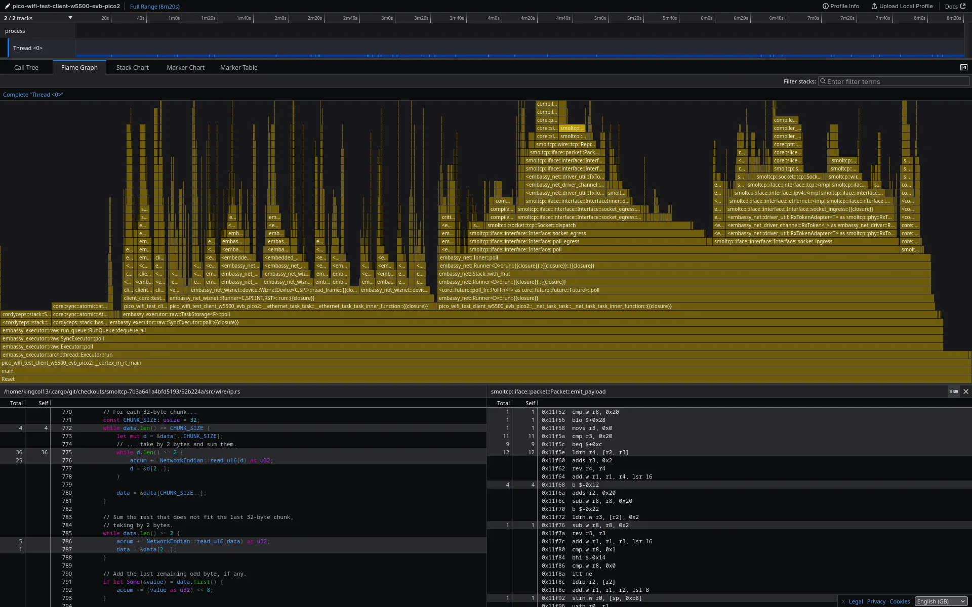
Flame graphs

The widths of the bars of the flamegraph are proportional to the number of samples and hence to the time spent in that function. The x-axis is sorted alphabetically. The y-axis is stack depth, from caller-most at the bottom to callee-most at the top. See this blog post for an introduction to flamegraphs.

Saving and sharing profiles

To correctly display the profile with samply, the sampled binary must be present at the <executing-elf-file> path. In order to embed the function names into a profile which you can then share with others, you can use the “Upload Local Profile” option in firefox profiler and then click “Download”.

Firefox profiler

Check the firefox profiler docs for more information on navigating the interface. The transforms section, detailing how to focus and merge, is particularly useful.